
NOTE: You do not have to “memorise” the code examples below, but you must get to a stage of fully understanding what each line of code is doing!
Big O Notation
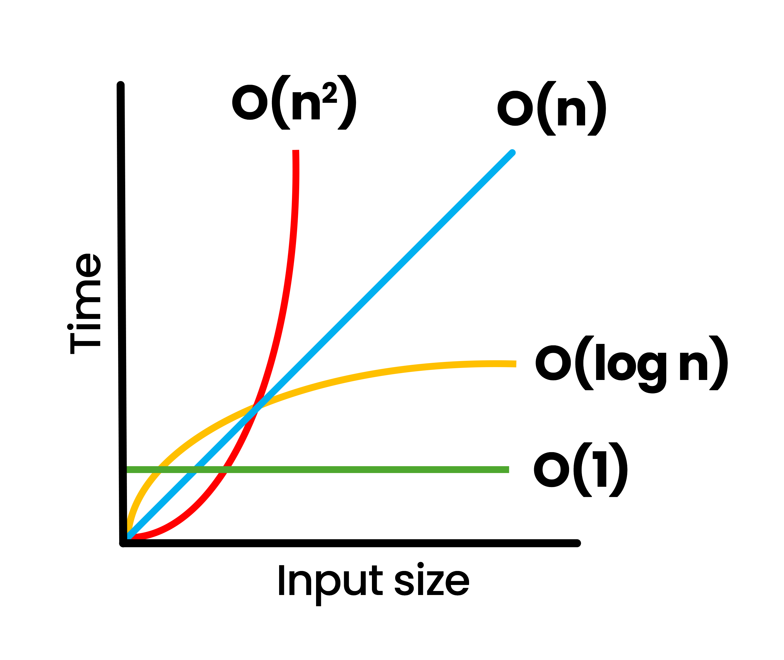
Big O notation is a mathematical concept used to describe and classify algorithms based on how their run time or space requirements grow as the size of the input increases. It identifies the efficiency of an algorithm.
Linear – O(n)
- The algorithm’s time or space complexity increases proportionally with the input size.
- Linear search: Often characterized by a single loop over the input data.
- Example: Finding an item in an unsorted list by checking each element one by one.
Logarithmic – O(log n)
- Complexity increases logarithmically, significantly faster than linear for large inputs.
- Binary Search: Typical example where the dataset is halved each step.
- Efficient Scaling: Performance degrades slowly as the input size increases.
Constant – O(1)
- The operation takes the same amount of time or space regardless of input size.
- Direct Access: Examples include accessing an array element by index.
- No Loops: No use of loops or recursive calls that depend on the input size.
Quadratic – O(n²)
- Performance is proportional to the square of the input size.
- Nested Loops: Typically found in algorithms with two nested loops over the input data.
- Slow: Becomes impractical for large inputs due to the rapid increase in time or space required.
Search Algorithms
Linear Search
Linear search algorithm iterates over all elements in the list and checks if the element is equal to the target value.
# O(n) linear time complexity
def linear_search(lst, target):
    for i in range(len(lst)):
        if lst[i] == target:
            return i
    return -1 # if target is not found

def main():
    index = linear_search([1, 3, 5, 7, 9, 11, 13, 15, 17, 19], 11)
    # index will be 5
    print(index)
Binary Search
Binary search is an efficient algorithm for finding an item from a sorted list of items. It repeatedly divides in half the portion of the list that could contain the item, until you’ve narrowed down the possible locations to just one.
# O(log n) logarithmic time complexity
def binary_search(lst, target):
    low = 0
    high = len(lst) - 1

    while low <= high:
        mid = (low + high) // 2 # Two // rounds the division down
        guess = lst[mid]
        if guess == target:
            return mid  # Target found, return index
        elif guess > target:
            high = mid - 1  # Target is in the left half
        else:
            low = mid + 1  # Target is in the right half

    return -1  # Target is not in the list

def main():
    sorted_list = [1, 3, 5, 7, 9, 11, 13, 15, 17, 19]
    target_value = 11

    index = binary_search(sorted_list, target_value)
    if index != -1:
        print(f"Target found at index: {index}")
    else:
        print("Target not found in the list.")
Sort Algorithms
Bubble Sort
Bubble sort is a sorting algorithm that repeatedly steps through the list, compares adjacent elements, and swaps them if they are in the wrong order. The algorithm gets its name because smaller elements “bubble” to the top of the list.
# O(n^2) quadratic time complexity
def bubble_sort(lst):
  n = len(lst)
  for i in range(n):
    for j in range(0, n - i - 1):
      if lst[j] > lst[j + 1]:
        temp = lst[j]
        lst[j] = lst[j+1]
        lst[j+1] = temp
  return lst

def main():
  sorted_list = bubble_sort([64, 34, 25, 12, 22, 11, 90])
  print(sorted_list)  # Output will be [11, 12, 22, 25, 34, 64, 90]
Insertion Sort
Insertion sort is a simple sorting algorithm that builds the final sorted array one item at a time by comparing each new element to the already sorted portion and inserting it into the correct position.
# O(n^2) quadratic time complexity
def insertion_sort(lst):
    for i in range(1, len(lst)):
        key = lst[i]
        j = i - 1

        while j >= 0 and key < lst[j]:
            lst[j + 1] = lst[j]
            j -= 1

        lst[j + 1] = key

    return lst

def main():
  sorted_list = insertion_sort([64, 34, 25, 12, 22, 11, 90])
  # sorted_list will be [11, 12, 22, 25, 34, 64, 90]
Selection Sort
Selection sort divides the input list into two parts: a sorted sublist of items which is built up from left to right at the front (left) of the list, and a sublist of the remaining unsorted items. On each iteration, the smallest (or largest, depending on sorting order) remaining element from the unsorted sublist is found and moved to the end of the sorted sublist.
# O(n^2) quadratic time complexity
def selection_sort(lst):
  n = len(lst)
  for i in range(n):
    # Find the minimum element in remaining unsorted array
    min_idx = i
    for j in range(i + 1, n):
      if lst[min_idx] > lst[j]:
        min_idx = j
    # Swap the found minimum element with the first element
    temp = lst[i]
    lst[i] = lst[min_idx]
    lst[min_idx] = temp
  return lst

def main():
  sorted_list = selection_sort([64, 34, 25, 12, 22, 11, 90])
  # sorted_list will be [11, 12, 22, 25, 34, 64, 90]
  print(sorted_list)